ECL calculation methodology

Credit Risk Suite – Expected Credit Losses Methodology article

Introduction

The IFRS 9 accounting standard has been effective since 2018 and affects both financial institutions and corporates. Although the IFRS 9 standards are principle-based and simple, the design and implementation can be challenging. Specifically, the difficulties that the incorporation of forward-looking information in the loss estimate introduces should not be underestimated. Using our hands-on experience and over two decades of credit risk expertise of our consultants, Zanders developed the Credit Risk Suite. The Credit Risk Suite is a calculation engine that determines transaction-level IFRS 9 compliant provisions for credit losses. The CRS was designed specifically to overcome the difficulties that our clients face in their IFRS 9 provisioning. In this article, we will elaborate on the methodology of the ECL calculations that take place in the CRS.

An industry best-practice approach for ECL calculations requires four main ingredients:

• Probability of Default (PD): The probability that a counterparty will default at a certain point in time. This can be a one-year PD, i.e. the probability of defaulting between now and one year, or a lifetime PD, i.e. the probability of defaulting before the maturity of the contract. A lifetime PD can be split into marginal PDs which represent the probability of default in a certain period.
• Exposure at Default (EAD): The exposure remaining until maturity of the contract based on current exposure, contractual, expected redemptions and future drawings on remaining commitments.
• Loss Given Default (LGD): The percentage of EAD that is expected to be lost in case of default. The LGD differs with the level of collateral, guarantees and subordination associated with the financial instrument.
• Discount Factor (DF): The expected loss per period is discounted to present value terms using discount factors. Discount factors according to IFRS 9 are based on the effective interest rate.

The overall ECL calculation is performed as follows and illustrated by the diagram below:

Model components

The CRS consists of multiple components and underlying models that are able to calculate each of these ingredients separately. The separate components are then combined into ECL provisions which can be utilized for IFRS 9 accounting purposes. Besides this, the CRS contains a customizable module for scenario-based Forward-Looking Information (FLI). Moreover, the solution allocates assets to one of the three IFRS 9 stages. In the component approach, projections of PDs, EADs and LGDs are constructed separately. This component-based setup of the CRS allows for customizable and easy to implement approach. The methodology that is applied for each of the components is described below.

Probability of default

For each projected month, the PD is derived from the PD term structure that is relevant for the portfolio as well as the economic scenario. This is done using the PD module. The purpose of this module is to determine forward-looking Point-in-Time (PIT) PDs for all counterparties. This is done by transforming Through-the-Cycle (TTC) rating migration matrices into PIT rating migration matrices. The TTC rating migration matrices represent the long-term average annual transition PDs, while the PIT rating migration matrices are annual transition PDs adjusted to the current (expected) state of the economy. The PIT PDs are determined in the following steps:

1. Determine TTC rating transition matrices: To be able to calculate PDs for all possible maturities, an approach based on rating transition matrices is applied. A transition matrix specifies the probability to go from a specified rating to another rating in one year time. The TTC rating transition matrices can be constructed using e.g., historical default data provided by the client or external rating agencies.
2. Apply forward-looking methodology: IFRS 9 requires the state of the economy to be reflected in the ECL. In the CRS, the state of the economy is incorporated in the PD by applying a forward-looking methodology. The forward-looking methodology in the CRS is based on a ‘Z-factor approach’, where the Z-factor represents the state of the macroeconomic environment. Essentially, a relationship is determined between historical default rates and specific macroeconomic variables. The approach consists of the following sub-steps:
   1. Derive historical Z-factors from (global or local) historical default rates.
   2. Regress historical Z-factors on (global or local) macro-economic variables.
   3. Obtain Z-factor forecasts using macro-economic projections.
3. Convert rating transition matrices from TTC to PIT: In this step, the forward-looking information is used to convert TTC rating transition matrices to point-in-time (PIT) rating transition matrices. The PIT transition matrices can be used to determine rating transitions in various states of the economy.
4. Determine PD term structure: In the final step of the process, the rating transition matrices are iteratively applied to obtain a PD term structure in a specific scenario. The PD term structure defines the PD for various points in time.

The result of this is a forward-looking PIT PD term structure for all transactions which can be used in the ECL calculations.

Exposure at default

For any given transaction, the EAD consists of the outstanding principal of the transaction plus accrued interest as of the calculation date. For each projected month, the EAD is determined using cash flow data if available. If not available, data from a portfolio snapshot from the reporting date is used to determine the EAD.

Loss given default

For each projected month, the LGD is determined using the LGD module. This module estimates the LGD for individual credit facilities based on the characteristics of the facility and availability and quality of pledged collateral. The process for determining the LGD consists of the following steps:

1. Seniority of transaction: A minimum recovery rate is determined based on the seniority of the transaction.
2. Collateral coverage: For the part of the loan that is not covered by the minimum recovery rate, the collateral coverage of the facility is determined in order to estimate the total recovery rate.
3. Mapping to LGD class: The total recovery rate is mapped to an LGD class using an LGD scale.

Scenario-weighted average expected credit loss

Once all expected losses have been calculated for all scenarios, the weighted average one-year and lifetime loss are calculated for each transaction , for both 1-year and lifetime scenario losses:

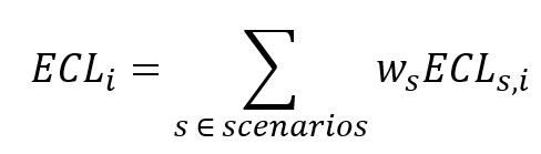
For each scenario , the weights  are predetermined. For each transaction , the scenario losses are weighted according to the formula above, where  is either the lifetime or the one-year expected scenario loss. An example of applied scenarios and corresponding weights is as follows:

• Optimistic scenario: 25%
• Neutral scenario: 50%
• Pessimistic scenario: 25%

This results in a one-year and a lifetime scenario-weighted average ECL estimate for each transaction.

Stage allocation

Lastly, using a stage allocation rule, the applicable (i.e., one-year or lifetime) scenario-weighted ECL estimate for each transaction is chosen. The stage allocation logic consists of a customisable quantitative assessment to determine whether an exposure is assigned to Stage 1, 2 or 3. One example could be to use a relative and absolute PD threshold:

• Relative PD threshold: +300% increase in PD (with an absolute minimum of 25 bps)
• Absolute PD threshold: +3%-point increase in PD The PD thresholds will be applied to one-year best estimate PIT PDs.

If either of the criteria are met, Stage 2 is assigned. Otherwise, the transaction is assigned Stage 1.

The provision per transaction are determined using the stage of the transaction. If the transaction stage is Stage 1, the provision is equal to the one-year expected loss. For Stage 2, the provision is equal to the lifetime expected loss. Stage 3 provision calculation methods are often transaction-specific and based on expert judgement.